Rossby Wave Packet Diagnostics (Ghinassi et al. 2018)

A reproduction of the results of section 4, Large-amplitude Rossby wave packets in an idealized barotropic model simulation, by Ghinassi et al. (2018).

import numpy as np
import matplotlib.pyplot as plt
import barotropic as bt

Model setup and integration

# 2° resolution of longitude-latitude grid
grid = bt.Grid(resolution=2.)
# No forcing
rhs = None
# Model with hyperdiffusion
model = bt.BarotropicModel(rhs, diffusion_order=2, diffusion_coeff=1.0e15)

# Start from Held and Phillips (1987) zonal profile
background_u = bt.init.held_1985(grid)

# Add perturbation according to eqs. (24) to (26)
# λ_2 = 3π/2 here instead of 2π/3 as in the paper, which seems to be a typo
def perturbation_vorticity(grid, s1, s2, zeta0, phi0, lam1, lam2, sigma_phi, sigma_lam):
    L1 = np.exp(-((grid.lam2 - lam1)/sigma_lam)**2) * np.sin(s1 * grid.lam2)
    L2 = np.exp(-((grid.lam2 - lam2)/sigma_lam)**2) * np.cos(s2 * grid.lam2)
    return zeta0 * np.cos(grid.phi2) * np.exp(-((grid.phi2 - phi0)/sigma_phi)**2) * (L1 + L2)

perturbation = perturbation_vorticity(grid, s1=6, s2=9, zeta0=8.0e-5, phi0=np.pi/4,
        lam1=np.pi/3, lam2=3*np.pi/2, sigma_phi=np.deg2rad(10), sigma_lam=np.deg2rad(30))

# Add vorticity perturbation to background state to obtain initial state
init = background_u.add_vorticity(perturbation)

# Run model for 5 days with a timestep of 900 seconds and save state every 24 hours
last, states = model.run(init, 900, 5*bt.DAY, save_every=1*bt.DAY)

Figure 5

Absolute vorticity in the barotropic model simulation (a) at initial time and (b) after 5 days of integration.

def style_lonlat(ax):
    ax.set_xticks([0, 60, 120, 180, 240, 300])
    ax.set_xticklabels(["0°", "60°E", "120°E", "180°", "120°W", "60°W"])
    ax.set_ylim([0, 90])
    ax.set_yticks([0, 10, 20, 30, 40, 50, 60, 70, 80])
    ax.set_yticklabels(["0°", "10°N", "20°N", "30°N", "40°N", "50°N", "60°N", "70°N", "80°N"])
    ax.grid(linestyle="dotted", color="k")

fig, (ax1, ax2, ax3) = plt.subplots(3, 1, figsize=(6, 5), gridspec_kw=dict(height_ratios=(8, 8, 1)))

pv_levels = [0.2, 0.4, 0.6, 0.8, 1.0, 1.2, 1.4, 1.6]
pv_cmap = "viridis"

ax1.set_title("(a)", loc="left")
ax1.set_title("Absolute vort (t = {:.0f} h)".format(init.time / bt.HOUR), loc="center")
ax1.contourf(grid.lon2, grid.lat2, init.pv * 10000,
             levels=pv_levels, cmap=pv_cmap, extend="both")
style_lonlat(ax1)

ax2.set_title("(b)", loc="left")
ax2.set_title("Absolute vort (t = {:.0f} h)".format(last.time / bt.HOUR), loc="center")
pv2 = ax2.contourf(grid.lon2, grid.lat2, last.pv * 10000,
                   levels=pv_levels, cmap=pv_cmap, extend="both")
plt.colorbar(pv2, cax=ax3, orientation="horizontal")
ax3.set_title("$10^{-4}\;\mathrm{s}^{-1}$", loc="right")
style_lonlat(ax2)

fig.tight_layout()

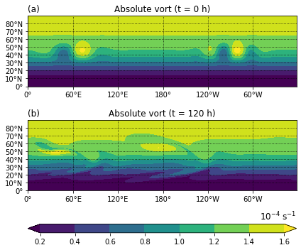
Figure 6

Evolution of (left) filtered LWA and (right) the envelope of the meridional wind in the barotropic model simulation, shown as snapshots every 24h.

fig, axs = plt.subplots(7, 2, figsize=(10, 12), gridspec_kw=dict(height_ratios=(7, 7, 7, 7, 7, 7, 1)))

panels = list("lfkejdichbga")

for state, (axl, axr) in zip(states, axs):
    # State.falwa_filtered uses Fourier instead of wavelet transform to
    # obtain the dominant wavenumber, so compute manually here
    dominant_wavenumber = bt.diagnostics.dominant_wavenumber_wavelet(state.v, grid)
    falwa_filtered = bt.diagnostics.filter_by_wavenumber(state.falwa, 2*dominant_wavenumber)

    axl.set_title("(" + panels.pop() + ")", loc="left")
    axl.set_title("Filtered LWA (t = {:.0f}h)".format(state.time / bt.HOUR), loc="center")
    ml = axl.contourf(grid.lon2, grid.lat2, falwa_filtered,
                      levels=[0, 4, 8, 12, 16, 20], extend="max", cmap="YlOrRd")
    axr.set_title("(" + panels.pop() + ")", loc="left")
    axr.set_title("Envelope of v (t = {:.0f}h)".format(state.time / bt.HOUR), loc="center")
    mr = axr.contourf(grid.lon2, grid.lat2, state.v_envelope_hilbert,
                      levels=[4, 8, 12, 16, 20], extend="both", cmap="Purples")

plt.colorbar(ml, cax=axs[-1,0], orientation="horizontal")
plt.colorbar(mr, cax=axs[-1,1], orientation="horizontal")

axs[-1,0].set_title("$\mathrm{m}\;\mathrm{s}^{-1}$", loc="right")
axs[-1,1].set_title("$\mathrm{m}\;\mathrm{s}^{-1}$", loc="right")

for ax in axs[:-1,:].flatten():
    style_lonlat(ax)

fig.tight_layout()

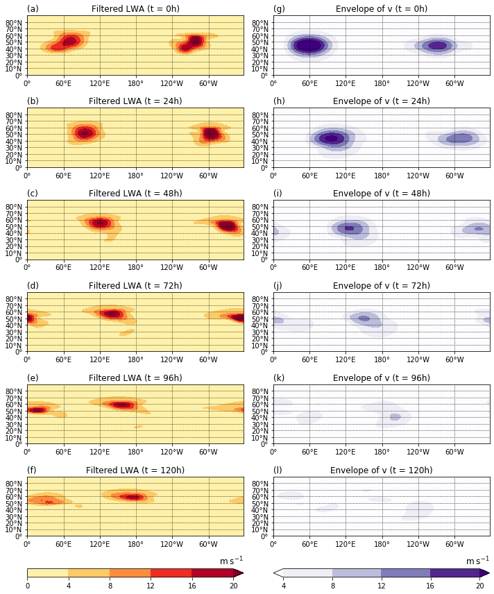
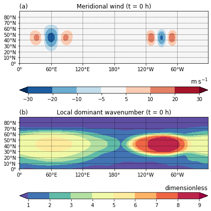
Figure A1

Initial state of the barotropic model simulation: (a) meridional wind \(v\) and (b) local dominant wavenumber from wavelet analysis.

fig, (ax1, ax2, ax3, ax4) = plt.subplots(4, 1, figsize=(6, 6), gridspec_kw=dict(height_ratios=(8, 1, 8, 1)))

ax1.set_title("(a)", loc="left")
ax1.set_title("Meridional wind (t = {:.0f} h)".format(init.time / bt.HOUR), loc="center")
m1 = ax1.contourf(grid.lon2, grid.lat2, init.v,
                  levels=[-30, -20, -10, -5, 5, 10, 20, 30], cmap="RdBu_r", extend="both")
plt.colorbar(m1, cax=ax2, orientation="horizontal")
ax2.set_title("$\mathrm{m}\;\mathrm{s}^{-1}$", loc="right")
style_lonlat(ax1)

ax3.set_title("(b)", loc="left")
ax3.set_title("Local dominant wavenumber (t = {:.0f} h)".format(init.time / bt.HOUR), loc="center")
m3 = ax3.contourf(grid.lon2, grid.lat2, bt.diagnostics.dominant_wavenumber_wavelet(init.v, grid),
                  levels=[1, 2, 3, 4, 5, 6, 7, 8, 9], cmap="Spectral_r", extend="both")
plt.colorbar(m3, cax=ax4, orientation="horizontal")
ax4.set_title("dimensionless", loc="right")
style_lonlat(ax3)

fig.tight_layout()